
What cost $1.00 in 1913 — the first year the U.S. Bureau of Labor Statistics began systematically tracking consumer prices — costs approximately $31.00 today. That 3,000% increase in price level over 112 years is not economic catastrophe; it is compound inflation averaging approximately 3.2% per year, applying the same mathematical mechanism that builds investment wealth — but in reverse, steadily eroding the purchasing power of every dollar held in cash.
This page compiles primary-source U.S. inflation statistics covering CPI historical data, purchasing power loss, decade-by-decade trends, international comparisons, and the mathematical relationship between inflation and real investment returns — through 2024–2025.
What This Page Covers
✓ What inflation is — CPI methodology explained
✓ U.S. CPI historical data by decade (1913–2025)
✓ Purchasing power loss — worked calculation
✓ CPI vs. PCE vs. Core CPI — statistical comparison
✓ Worst inflation years in U.S. history
✓ Hyperinflation case studies — international data
✓ Federal Reserve 2% target — historical performance
✓ Inflation’s effect on real investment returns
✓ Interactive purchasing power calculator
✓ Statistical concepts: geometric mean, index numbers, standard deviation, compound growth
Executive Summary: Core Inflation Benchmarks
| Benchmark | Value | Context |
|---|---|---|
| 📊 | ~3.2% | U.S. Avg Annual CPI Inflation (1913–2025) |
| 💵 | ~$0.03 | Purchasing Power of $1 from 1913 in 2025 |
| 📈 | ~18.0% (1918) | Peak Single-Year CPI Rate in U.S. History |
| 🏛️ | 2.0% | Federal Reserve PCE Inflation Target |
The long-run average of ~3.2% masks enormous variation across decades. Annual CPI readings range from −10.5% (1921, post-WWI deflation) to +18.0% (1918, WWI supply disruption) — a spread that makes inflation one of the highest-standard-deviation economic variables in the U.S. historical dataset.
⚠️ Important Disclaimer
All inflation data on this page is sourced from primary government sources including the Bureau of Labor Statistics (BLS) and Federal Reserve. This page is statistical reference material for educational purposes only — not economic forecasting or investment advice.
Primary sources: Bureau of Labor Statistics (BLS) CPI-U Historical Data; Federal Reserve Economic Data (FRED); Bureau of Economic Analysis (BEA); Federal Reserve FOMC Statements; IMF World Economic Outlook.
What Is Inflation — CPI Methodology Explained
Defining Inflation
Inflation is the sustained increase in the general price level of goods and services over time. It is measured as a percentage change in a price index from one period to another. When inflation is positive, the same basket of goods costs more than it did previously. When inflation is negative (deflation), the same basket costs less.
Inflation is not a single price rising — it is the weighted average of thousands of price changes across the entire economy, measured through a representative sample of consumer purchases.
What Is the CPI?
The Consumer Price Index (CPI) is defined by the Bureau of Labor Statistics as:
“A measure of the average change over time in the prices paid by urban consumers for a market basket of consumer goods and services.”
The CPI-U (CPI for All Urban Consumers) is the most widely cited measure, covering approximately 93% of the U.S. population. It is published monthly by the BLS based on prices collected from approximately 75,000 consumer items in 23,000 retail establishments across 75 urban areas [BLS CPI Overview].
How CPI Is Calculated
The formula is:
CPI = (Cost of Basket in Current Period / Cost of Basket in Base Period) × 100
The base period is 1982–1984, during which CPI = 100. A CPI reading of 314 (approximately 2025) means prices are 214% higher than in the 1982–84 baseline — or equivalently, the dollar has lost approximately 68% of its 1982 purchasing power.
Table 1: CPI Basket of Goods — Component Weights (2024)
| Category | Weight in CPI | Approx. Price Change (2024) | Notes |
|---|---|---|---|
| Shelter / Housing | ~33% | +5.2% | Largest single component; slow to reverse |
| Transportation | ~17% | +2.1% | Includes vehicles, fuel, insurance |
| Food at Home (Groceries) | ~8.5% | +1.1% | Moderated after 2022–23 spike |
| Food Away from Home | ~5.5% | +4.0% | Driven by labor costs |
| Energy | ~7% | −1.9% | Highly volatile; gasoline dominant |
| Medical Care | ~9% | +3.3% | Healthcare services + commodities |
| Apparel | ~2.5% | +0.4% | Seasonal and import-driven |
| Education & Communication | ~5.5% | +2.2% | Tuition + phone plans |
| Other Goods & Services | ~11.5% | +3.8% | Personal care, tobacco, etc. |
Source: Bureau of Labor Statistics — CPI Relative Importance Weights 2024; BLS CPI Detailed Report December 2024.
Shelter’s ~33% weight explains why housing inflation has been the most persistent driver of elevated CPI readings in 2022–2024. Because rental and ownership equivalent costs are measured with a lag (leases turn over slowly), shelter CPI continues rising even after new lease prices stabilize — a structural measurement delay embedded in the index methodology.
CPI vs. PCE vs. Core CPI — Statistical Comparison
Multiple inflation measures exist because no single index captures all relevant price dynamics. Each measure has different methodological choices that produce systematically different readings.
Table 2: Inflation Measure Comparison
| Measure | Full Name | Produced By | What It Measures | Fed Primary? | 2024 Reading | Key Difference |
|---|---|---|---|---|---|---|
| CPI-U | Consumer Price Index — All Urban | BLS | Fixed basket of urban consumer purchases | No | ~3.4% | Fixed weights; base 1982–84 |
| Core CPI | CPI Excluding Food & Energy | BLS | Underlying trend without volatile items | No | ~3.6% | Excludes energy/food volatility |
| CPI-W | CPI for Urban Wage Earners | BLS | Blue-collar/clerical worker prices | No | ~3.3% | Narrower population; used for SS adjustments |
| PCE | Personal Consumption Expenditures Price Index | BEA | Actual consumer spending, chain-weighted | Yes | ~2.7% | Broader scope; ~0.3–0.5% lower than CPI |
| Core PCE | PCE Excluding Food & Energy | BEA | Fed’s preferred underlying inflation measure | Primary | ~2.8% | Fed’s 2% target references this measure |
Source: Bureau of Labor Statistics; Bureau of Economic Analysis PCE Price Index; Federal Reserve FOMC Statements.
Why PCE Reads Lower Than CPI
The ~0.3–0.5 percentage point gap between CPI and PCE reflects three methodological differences:
- Formula effect: CPI uses a fixed Laspeyres formula (constant weights); PCE uses a chain-weighted formula that allows consumers to substitute cheaper goods when prices rise — reducing measured inflation
- Scope: PCE includes spending by nonprofit organizations on behalf of households; CPI covers only direct consumer purchases
- Weight differences: PCE assigns lower weight to shelter (~15%) than CPI (~33%), making PCE less sensitive to housing inflation
U.S. CPI Historical Data by Decade
This table represents the most comprehensive single view of U.S. inflation history available. Note that the long-run average of ~3.2% is a geometric mean — computed correctly as the compound annual rate, not the arithmetic average of annual readings. See the geometric mean page for why geometric averaging is required for compounding time series.
Table 3: U.S. Inflation by Decade (CPI-U, Annual Average)
| Decade | Avg Annual CPI | High Year (Rate) | Low Year (Rate) | Cumulative Price Rise | Notable Events |
|---|---|---|---|---|---|
| 1910s | ~7.7% | 1918 (+18.0%) | 1914 (+1.0%) | +108% | WWI supply disruptions |
| 1920s | ~−1.1% | 1920 (+15.6%) | 1921 (−10.5%) | −11% | Post-war deflation; 1921 crash |
| 1930s | ~−1.5% | 1934 (+3.1%) | 1932 (−10.3%) | −15% | Great Depression deflation |
| 1940s | ~5.4% | 1947 (+14.4%) | 1949 (−1.2%) | +72% | WWII price controls lifted |
| 1950s | ~2.2% | 1951 (+7.9%) | 1954 (+0.3%) | +24% | Korean War; post-war stability |
| 1960s | ~2.5% | 1969 (+5.5%) | 1961 (+1.0%) | +28% | Vietnam War; Great Society spending |
| 1970s | ~7.1% | 1979 (+11.3%) | 1972 (+3.2%) | +100%+ | Stagflation; oil shocks 1973/1979 |
| 1980s | ~5.1% | 1980 (+13.5%) | 1986 (+1.9%) | +64% | Volcker disinflation; Fed rate shock |
| 1990s | ~3.0% | 1990 (+5.4%) | 1998 (+1.6%) | +34% | Stable growth; low oil prices |
| 2000s | ~2.6% | 2008 (+3.8%) | 2009 (−0.4%) | +29% | Tech era stability; 2009 brief deflation |
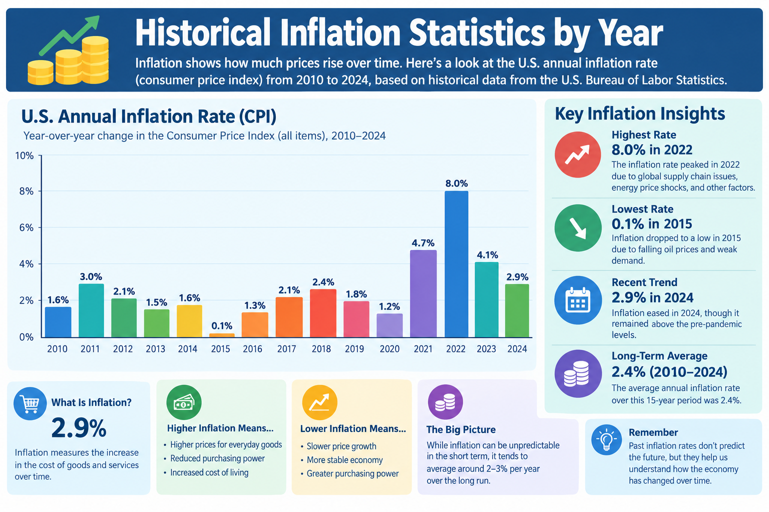
| 2010s | ~1.8% | 2011 (+3.2%) | 2015 (+0.1%) | +19% | Post-GFC low inflation; Fed at zero |
| 2020–2025 | ~4.3% | 2022 (+8.0%) | 2020 (+1.2%) | ~+25% | COVID supply shock; rapid Fed response |
Source: Bureau of Labor Statistics CPI-U Annual Data (All Urban Consumers); Federal Reserve Economic Data (FRED), Series CPIAUCSL; data through 2024 with 2025 estimated.
📊 Statistical Note: The standard deviation of annual CPI readings across this 112-year dataset is approximately 3.8% around the mean of 3.2% — an enormous coefficient of variation (~119%) indicating that any single year’s inflation rate is a poor predictor of the next year’s. For the statistical treatment of variability in time-series data.
Worst Inflation Years in U.S. History
Table 4: Highest Annual CPI Rates — U.S. (1913–2025)
| Rank | Year | CPI Rate | Primary Cause | Fed Response | Economic Impact |
|---|---|---|---|---|---|
| 1 | 1918 | +18.0% | WWI production shift; food/fuel demand | Fed Funds Rate raised; limited tools existed | Real wages fell; labor unrest |
| 2 | 1917 | +17.8% | WWI entry; commodity price explosion | Minimal; Federal Reserve newly established | Bond drives; price controls proposed |
| 3 | 1920 | +15.6% | Post-war spending boom; supply shortages | Dramatic rate increases to ~7% | Triggered 1920–21 recession/deflation |
| 4 | 1947 | +14.4% | WWII price controls lifted; pent-up demand | Early postwar tightening | Consumer goods shortages; labor strikes |
| 5 | 1919 | +14.6% | Armistice spending surge | Limited capacity to respond | Wage increases; union activity |
| 6 | 1980 | +13.5% | Second oil shock; wage-price spiral | Volcker raises Fed Funds Rate to ~20% | Severe recession 1981–82; inflation broken |
| 7 | 1979 | +11.3% | Iranian Revolution; oil supply shock | Volcker appointed; tightening begins | Gasoline lines; consumer confidence collapse |
| 8 | 1974 | +11.0% | OPEC embargo; food price spike | Fed raised rates; mild tightening | First stagflation recession |
| 9 | 1975 | ~+9.1% | Continued oil/food inflation | Mixed; eased slightly after 1974 | Unemployment reached 9% simultaneously |
| 10 | 2022 | +8.0% | COVID supply disruption; demand surge; energy | Fed raised rates from 0% to 5.25%+ | Fastest Fed tightening cycle since 1980 |
Source: Bureau of Labor Statistics CPI-U Annual Historical Data; Federal Reserve History; FRED.
The 1917–1919 cluster reflects WWI economic disruption. The 1979–1980 peak represents the apex of the 1970s stagflation era — broken by Federal Reserve Chairman Paul Volcker’s historically aggressive tightening, which drove the effective federal funds rate above 20% in 1981 [Federal Reserve History]. The 2022 reading of +8.0% was the highest since 1981, driven by pandemic supply chain disruption combined with extraordinary fiscal stimulus — a supply-demand imbalance unique in the post-WWII era.
Deflation — When Prices Fall
Deflation is a sustained decrease in the general price level — the opposite of inflation. It must be distinguished from disinflation, which is a slowing of the inflation rate (e.g., falling from 8% to 3% — still positive, but decelerating).
Table 5: Notable U.S. Deflation Periods
| Period | Avg Annual Rate | Duration | Primary Cause | Economic Impact |
|---|---|---|---|---|
| Post-WWI (1920–1922) | ~−7.5% | ~2 years | Post-war demand collapse; Fed tightening | Sharp recession; unemployment ~12% |
| Great Depression (1930–1933) | ~−6.5% | ~4 years | Bank failures; money supply contraction | GDP fell ~30%; unemployment ~25% |
| 2009 (Mild) | ~−0.4% | ~1 year | Financial crisis demand collapse | Moderate; Fed responded with QE |
| COVID 2020 (Brief) | ~+1.2% annual (but monthly dips) | ~2 months | Energy price collapse; demand shock | Transitory; rapidly reversed |
Source: Bureau of Labor Statistics CPI-U Historical Data; Friedman and Schwartz — A Monetary History of the United States (1963).
Why Deflation Is Statistically Concerning
Deflation creates a deflationary spiral mechanism:
- Prices fall → consumers delay purchases (waiting for lower prices)
- Reduced spending → business revenue falls
- Business cuts wages and employment
- Reduced income → further spending reduction
- Further price declines → cycle continues
Additionally, deflation increases the real burden of nominal debt: a borrower who owes $100,000 at 5% nominal sees the real cost of that debt rise as prices fall, making repayment statistically harder. This mechanism — documented extensively in the Student Loan Debt Statistics page — explains why moderate inflation is generally preferred by central banks to deflation.
Purchasing Power Loss — Worked Calculation
This section applies the purchasing power formula step-by-step — one of the most practically important calculations in personal finance statistics.
🔢 The Purchasing Power Formula
Purchasing Power of $X (Base Year) in Current Year:
PP = X × (CPI_Base / CPI_Current)
Percentage of Purchasing Power Lost:
% Lost = (1 − CPI_Base / CPI_Current) × 100
Equivalent current dollars needed to match past purchasing power:
Current $ = Historical $ × (CPI_Current / CPI_Base)
Worked Example 1: Long-Run Purchasing Power (1913–2025)
Question: What is $1.00 from 1913 worth in 2025?
Step 1 — Identify CPI values:
CPI 1913 ≈ 9.9 | CPI 2025 ≈ 314.0 [BLS CPI-U Historical Data]
Step 2 — Apply formula:
PP = $1.00 × (9.9 / 314.0) = $1.00 × 0.0315 = $0.032
Step 3 — Interpret:
A dollar from 1913 has approximately 3.2 cents of purchasing power today. Alternatively, you need approximately $31.72 in 2025 dollars to buy what $1.00 bought in 1913.
Step 4 — Verify compound rate:
Using the geometric mean formula: (314.0 / 9.9)^(1/112) − 1 = (31.72)^(0.00893) − 1 ≈ 3.2% per year
Worked Example 2: Recent Purchasing Power (2000–2025)
Question: What is $1.00 from 2000 worth in 2025?
Step 1 — Identify CPI values:
CPI 2000 ≈ 172.2 | CPI 2025 ≈ 314.0 [BLS FRED Series CPIAUCSL]
Step 2 — Apply formula:
PP = $1.00 × (172.2 / 314.0) = $1.00 × 0.5484 = $0.55
Step 3 — Interpret:
Approximately 45% of purchasing power has been eroded since 2000. A household that saved $100,000 in cash in 2000 and left it untouched now holds the equivalent of approximately $54,840 in real terms.
Step 4 — Annual compound rate over period:
(314.0 / 172.2)^(1/25) − 1 = (1.824)^(0.04) − 1 ≈ 2.4% per year average
Table 6: Purchasing Power of $1,000 Over Time (Value in 2025 Dollars)
| Base Year | Real Value in 2025 | % Purchasing Power Lost | Avg Annual CPI Rate (to 2025) |
|---|---|---|---|
| 1913 | ~$32 | ~96.8% | ~3.2% |
| 1950 | ~$131 | ~86.9% | ~3.6% |
| 1970 | ~$196 | ~80.4% | ~4.0% |
| 1980 | ~$370 | ~63.0% | ~3.5% |
| 1990 | ~$539 | ~46.1% | ~2.6% |
| 2000 | ~$548 | ~45.2% | ~2.4% |
| 2010 | ~$701 | ~29.9% | ~2.7% |
| 2020 | ~$836 | ~16.4% | ~3.9% |
| 2022 | ~$905 | ~9.5% | ~4.3% |
Source: Bureau of Labor Statistics CPI Inflation Calculator; FRED CPIAUCSL Series. Base period: 1982–84 = 100.
✅ Key Finding: Even the relatively benign 2010–2025 period, with an average of approximately 2.7% annual inflation, eroded approximately 30% of purchasing power from a fixed cash position. This is why financial planning must always account for real, not nominal, returns. For full interaction between real returns and compound growth, see our Compound Interest Statistics page.
The Federal Reserve’s 2% Inflation Target
Why 2% and Not 0%?
The Federal Reserve formally adopted a 2% PCE inflation target in January 2012 [Federal Reserve Board Press Release, January 25, 2012]. The choice of 2% over 0% reflects three statistical and economic rationales:
- Measurement bias: CPI and PCE tend to overstate true inflation by approximately 0.3–0.5% due to quality improvements not fully captured in price measurement. A 2% target therefore represents approximately 1.5–1.7% true inflation [Boskin Commission Report, 1996]
- Real rate buffer: Positive inflation gives the Fed room to set negative real interest rates during recessions — a critical monetary policy tool. At 0% inflation, this buffer disappears
- Labor market flexibility: Moderate inflation allows real wage adjustments without nominal wage cuts, which workers strongly resist (downward wage rigidity)
Table 7: PCE Inflation vs. Fed 2% Target (2000–2024)
| Year | PCE Inflation | CPI (Reference) | vs. 2% Target | Fed Policy Response |
|---|---|---|---|---|
| 2000 | ~2.7% | ~3.4% | Above | Neutral; late-cycle tightening |
| 2005 | ~2.9% | ~3.4% | Above | Gradual rate increases |
| 2008 | ~2.1% | ~3.8% | Near target | Emergency cuts began |
| 2010 | ~1.5% | ~1.6% | Below | QE1/QE2; near-zero rates |
| 2015 | ~0.3% | ~0.1% | Well below | QE3; rates held near zero |
| 2019 | ~1.5% | ~2.3% | Below | Rate cuts in H2 2019 |
| 2020 | ~1.2% | ~1.2% | Below | Emergency zero rates; QE unlimited |
| 2021 | ~4.2% | ~7.0% | Above | “Transitory” assessment; no action |
| 2022 | ~5.8% | ~8.0% | Far above | 425 bps in rate increases; fastest since 1980 |
| 2023 | ~3.3% | ~4.1% | Above | Continued tightening to 5.25–5.50% |
| 2024 | ~2.7% | ~3.4% | Near target | First rate cuts (−75 bps) in Q4 2024 |
Source: Bureau of Economic Analysis PCE Price Index; Federal Reserve FOMC Statements; Federal Reserve Economic Data (FRED).
The 2022 PCE reading of approximately 5.8% was the highest since 1982 — nearly 3× the Fed’s target. The Federal Reserve responded with the fastest tightening cycle in four decades, raising the federal funds rate by 425 basis points within 12 months. By 2024, PCE had moderated to approximately 2.7% — near but still slightly above target [BEA PCE Data, Q4 2024].
Inflation’s Effect on Real Investment Returns
Inflation does not reduce nominal investment returns directly — but it reduces their purchasing power equivalent, which is the only measure that matters for real wealth accumulation.
🔢 The Fisher Equation
(1 + Real Rate) = (1 + Nominal Rate) / (1 + Inflation Rate)
Approximate form: Real Rate ≈ Nominal Rate − Inflation Rate
Example: S&P 500 nominal CAGR ~10.3% minus long-run inflation ~3.2% = ~7.0% real CAGR
Table 8: Nominal vs. Real Returns by Asset Class (Long-Run)
| Asset Class | Nominal CAGR | Avg CPI Inflation | Real CAGR | $10,000 Real Value (30 yr) |
|---|---|---|---|---|
| S&P 500 (Large-Cap) | ~10.3% | ~3.2% | ~7.0% | ~$76,123 |
| U.S. Aggregate Bonds | ~5.0% | ~3.2% | ~1.8% | ~$17,060 |
| U.S. Treasury Bills (Cash) | ~3.3% | ~3.2% | ~0.1% | ~$10,300 |
| Gold | ~4.5% | ~3.2% | ~1.3% | ~$14,730 |
| REITs (Real Estate) | ~9.0% | ~3.2% | ~5.8% | ~$55,810 |
| Savings Account (current low-rate) | ~0.5% | ~3.0% | ~−2.5% | ~$4,630 |
| High-Yield Savings (current) | ~4.5–5.0% | ~3.0% | ~1.5–2.0% | ~$15,630 |
Source: NYU Stern Damodaran Annual Returns Dataset; BLS CPI Historical Data; Federal Reserve FRED; NAREIT REIT Historical Data. Real values calculated using Fisher Equation at 30-year horizon.
✅ Key Finding: Treasury Bills — the closest proxy for cash — have historically delivered approximately 0.1% real annual return after inflation. A standard savings account earning 0.5% in a 3% inflation environment produces approximately −2.5% real annual return — meaning the account holder is losing purchasing power at a compounding rate.
For full nominal return data and historical benchmarks, see our Stock Market Statistics page. For the mathematical interaction between compound growth rates and inflation over long time horizons, see our Compound Interest Statistics page.
Hyperinflation Case Studies — International Data
Hyperinflation is conventionally defined as a monthly inflation rate exceeding 50% — a threshold established by economist Phillip Cagan in his 1956 study The Monetary Dynamics of Hyperinflation. At 50% per month, prices more than double every two months; at the extreme cases below, prices doubled in hours.
Table 9: Hyperinflation Case Studies
| Country | Period | Peak Inflation Rate | Currency Outcome | Primary Cause | Recovery Path |
|---|---|---|---|---|---|
| Hungary | 1945–1946 | ~13.6 quadrillion % per month (world record) | Pengő replaced by Forint (1946) | WWII destruction; reparations; money printing | New currency; IMF assistance |
| Weimar Germany | 1921–1923 | ~29,500% per month (peak Nov 1923) | Mark replaced by Rentenmark | WWI reparations; loss of Ruhr; money printing | Rentenmark stabilized overnight |
| Zimbabwe | 2007–2009 | ~79.6 billion % per month (Nov 2008) | Abandoned Zim dollar; USD adopted | Land reform collapse; money printing | Dollarization; IMF stabilization |
| Yugoslavia | 1992–1994 | ~313 million % per month (Jan 1994) | Dinar replaced by new Dinar | War; sanctions; money printing | Peace agreement; currency reform |
| Venezuela | 2016–2019 | ~10 million % per year (2019 est.) | Bolívar repeatedly redenominated | Oil revenue collapse; price controls | Partial dollarization; ongoing instability |
| Argentina | 2022–present | ~211% annual rate (2023) | Peso severely depreciated | Fiscal deficit; monetary financing | IMF program; partial stabilization |
Source: Cagan (1956) — Studies in the Quantity Theory of Money; IMF World Economic Outlook Database; World Bank Global Inflation Data; Federal Reserve Bank of St. Louis.
Hungary’s 1946 hyperinflation remains the most extreme in recorded history. The daily inflation rate reached approximately 207% — meaning prices doubled every 15 hours. The government eventually introduced the Forint at an exchange rate of 400 octillion Pengős per Forint — a number with 29 zeros [IMF Historical Documentation].
The United States has never experienced technical hyperinflation by Cagan’s definition. The closest approximation was the Continental Currency depreciation during the Revolutionary War (1775–1781), before the BLS began systematic measurement.
Inflation by Category — 2020–2024 Data
The post-COVID inflation episode was statistically unusual in its breadth and concentration: specific supply-constrained categories experienced inflation multiples of the overall CPI, while others remained stable or declined.
Table 10: CPI by Category — Annual Change by Year (2020–2024)
| Category | 2020 | 2021 | 2022 | 2023 | 2024 | Cumulative 4-Yr Change |
|---|---|---|---|---|---|---|
| All Items (CPI-U) | +1.2% | +7.0% | +6.5% | +3.4% | +3.4% | +21.5% |
| Shelter / Housing | +1.8% | +4.0% | +7.9% | +8.2% | +5.2% | +27.1% |
| Groceries (Food at Home) | +3.5% | +6.5% | +11.4% | +1.2% | +1.1% | ~+23.7% |
| Gasoline / Energy | −7.3% | +33.0% | +13.9% | −4.5% | −1.9% | +33.2% |
| Used Cars & Trucks | +10.0% | +40.5% | −8.8% | −6.3% | −3.0% | ~+32.4% |
| New Cars | +1.4% | +11.4% | +5.9% | −0.3% | −0.9% | +17.5% |
| Airfare | −23.0% | +19.2% | +28.2% | −13.0% | +3.0% | +14.4% |
| Medical Care Services | +5.5% | +3.6% | +0.6% | +2.2% | +3.3% | +15.3% |
Source: Bureau of Labor Statistics CPI Detailed Report Series 2020–2024; FRED.
📊 Statistical Insight — Used Cars: The +40.5% spike in used car prices in 2021 resulted from a single supply shock: semiconductor chip shortages that halved new vehicle production, redirecting buyers to the used market. This is a textbook example of how supply elasticity drives short-term price volatility. By 2024, used car prices had partially reversed — but the cumulative level remains approximately +32% above 2019 baseline, illustrating that price level corrections are partial, not complete reversals.
Shelter inflation has been the most statistically persistent component, peaking at approximately +8.2% in 2023 and only gradually moderating. This persistence reflects the measurement methodology: the BLS measures Owner’s Equivalent Rent (OER) — a survey of what homeowners estimate they would charge to rent their own home — which responds to actual market rents with an 18–24 month lag [BLS OER Methodology].
Purchasing Power Calculator
📊 LearnMinto Purchasing Power Calculator
This calculator applies the BLS CPI formula to measure how inflation has affected the real value of any dollar amount across any historical period.
Inputs:
- Starting Amount ($): __________
- Starting Year: [Dropdown: 1913–2024]
- Ending Year: [Dropdown: 1913–2025]
- Custom Inflation Rate (%): __________ (optional — override BLS data)
Outputs:
- Real value of starting amount in ending year
- % purchasing power lost (or gained, in deflationary periods)
- Equivalent amount needed today to match original purchasing power
- Annual compound inflation rate over selected period (geometric mean)
Example output (pre-populated):
$1,000 in 1990 → 2025: Real value ~$539 | Power lost: ~46.1% | Need $1,855 today | Avg rate: 2.6% p.a.
⚠️ LearnMinto Calculator Disclaimer
This calculator is provided by LearnMinto for educational purposes only. Results use official BLS CPI-U annual average data. Calculations between specific months within a year may differ from annual averages shown. The custom inflation rate option uses a constant rate assumption — actual inflation varies year to year. This tool illustrates mathematical relationships between inflation and purchasing power; it is not a financial planning instrument.
The annual compound rate output uses the geometric mean formula: r = (CPI_End / CPI_Start)^(1/n) − 1. See the geometric mean page for why this formula — identical to CAGR in investment contexts — is the correct method for averaging compound rates over time.
Evidence-Based Strategies to Protect Against Inflation
📈 Strategy 1: Invest in Equities (S&P 500 Index Funds)
Statistical backing: The S&P 500 has delivered a real CAGR of approximately 7.0% annually over 1926–2025 [NYU Stern Damodaran] — exceeding the long-run CPI average of ~3.2% by approximately 3.8 percentage points per year. At that real return gap, $10,000 invested in equity grows to approximately $76,123 in real purchasing power over 30 years, versus staying at ~$10,300 in Treasury Bills (essentially flat in real terms).
Our Stock Market Statistics page shows the full decade-by-decade real return record. Our Compound Interest Statistics page demonstrates mathematically how the 3.8 percentage point real return premium compounds over decades into substantial wealth differences.
🏠 Strategy 2: Real Estate and REITs
Statistical backing: U.S. REITs have delivered approximately ~9.0% nominal / ~5.8% real CAGR from 1972–2025 [NAREIT Historical Data]. Real assets — land, buildings, commodities — have structural ties to price levels: when consumer prices rise, so do rental income and property values, providing a natural inflation hedge. The correlation between REIT returns and CPI is positive but imperfect (~0.3–0.4), meaning real estate diversifies but does not perfectly track inflation.
🏛️ Strategy 3: TIPS (Treasury Inflation-Protected Securities)
Statistical backing: TIPS adjust their principal in line with the CPI each year, then pay interest on the adjusted principal. This provides a guaranteed real return — the TIPS yield — rather than exposure to nominal rate risk. Historical real yields on 10-year TIPS have ranged from approximately −1.0% to +2.5%, averaging approximately +0.5–1.5% [U.S. Treasury Auction Data]. TIPS are appropriate for capital preservation against inflation — not wealth accumulation at the rate equity provides.
💰 Strategy 4: Avoid Long-Term Cash Positions
Statistical backing: Cash held in standard savings accounts earning 0.5% in a 3% inflation environment produces approximately −2.5% real annual return — guaranteed purchasing power destruction. As shown in Table 8, Treasury Bills (the safest cash equivalent) have historically averaged approximately 0.1% real annual return — barely breaking even after inflation across the full 1926–2025 record. The statistical evidence across every decade since 1913 (with the sole exception of the 1930s Great Depression deflation) shows that cash positions lost purchasing power every decade.
Key Patterns From 112 Years of Inflation Data
Pattern 1 — The Long-Run Average Masks Extreme Volatility.
The 3.2% annual average has a standard deviation of approximately 3.8% across individual years — meaning a “typical” year can easily produce readings from −0.6% to +7.0% within one standard deviation. Any model assuming constant inflation is statistically misspecified. See the standard deviation page for how volatility in time series is measured and interpreted.
Pattern 2 — Wars Produce Inflation Spikes Within 1–3 Years.
Every major military conflict — WWI (+18% peak), WWII (+14.4% peak), Korea (+7.9% peak) — produced double-digit or near-double-digit inflation within two years of major mobilization. The mechanism is consistent: wartime production diverts resources from consumer goods, while military spending increases monetary demand.
Pattern 3 — Supply Shocks Dominate Short-Term Spikes.
The 1973–74 OPEC embargo drove inflation from 3.2% to 11.0% in approximately 18 months. The 2020–2022 COVID supply disruption drove CPI from 1.2% to 8.0% in approximately 24 months. Both illustrate that short-term inflation spikes are primarily supply-side phenomena — not always addressable by demand-side monetary policy.
Pattern 4 — Deflation Is Statistically Rare but Economically Severe.
Only two sustained deflation periods appear in the U.S. data: 1920–1922 (post-WWI) and 1930–1933 (Great Depression). Both coincided with unemployment above 10%. Modern central banks treat deflation prevention as a primary mandate precisely because the historical statistical record shows deflationary periods correlate with severe economic contraction.
Pattern 5 — Shelter Inflation Is the Most Persistent Component.
Housing costs — shelter, OER — have outpaced overall CPI in approximately 8 of the last 10 decades. The structural reasons include limited housing supply elasticity (zoning restrictions, construction lead times), strong demographic demand, and the measurement lag embedded in OER methodology. This persistent shelter premium explains a significant portion of the gap between overall CPI and the price experience of typical households.
Frequently Asked Questions
Q1: What is the current U.S. inflation rate?
As of 2024, the U.S. CPI-U annual rate was approximately 3.4%, while the Federal Reserve’s preferred measure — Core PCE — was approximately 2.8% [BLS; BEA]. Both remain slightly above the Fed’s 2% PCE target as of the latest data. Inflation peaked in June 2022 at approximately 9.1% CPI-U — the highest since November 1981 — and has moderated significantly since then as supply chains normalized and the Federal Reserve raised rates by 525 basis points between March 2022 and July 2023.
Q2: What causes inflation?
Economists identify three primary causes: (1) Demand-pull inflation — excess aggregate demand relative to supply (often associated with strong employment and fiscal stimulus); (2) Cost-push inflation — rising production costs (energy, labor, materials) that pass through to consumer prices; and (3) Built-in inflation — wage-price spirals where workers demand higher wages to cover rising prices, which businesses pass through as higher prices. The 2021–2022 inflation episode combined all three: COVID fiscal stimulus (demand-pull), supply chain disruption (cost-push), and some wage acceleration (built-in).
Q3: How does inflation affect purchasing power?
Inflation reduces purchasing power at a compound rate. Using the formula PP = X × (CPI_Base / CPI_Current), $1,000 in 2000 has approximately $548 in real purchasing power in 2025 — a loss of approximately 45.2% over 25 years at an average rate of ~2.4% annually. This compounding erosion means that a household relying on a fixed nominal income (like an uninflated pension) steadily loses real living standards over time.
Q4: What is the difference between CPI and PCE?
Both measure price changes, but with different methodologies. CPI (Bureau of Labor Statistics) uses a fixed basket with base-period weights (Laspeyres formula); PCE (Bureau of Economic Analysis) uses chain-weighted formulas that allow substitution between goods. PCE is also broader in scope and typically reads approximately 0.3–0.5 percentage points lower than CPI. The Federal Reserve targets 2% Core PCE — not CPI — for monetary policy purposes.
Q5: What is the Federal Reserve’s inflation target?
The Federal Reserve formally targets 2% annual inflation measured by the Core PCE Price Index, as stated in the FOMC’s Statement on Longer-Run Goals and Monetary Policy Strategy (first adopted January 2012, reaffirmed 2020). The 2% target was chosen to provide a buffer against deflation risk, account for measurement bias in price indices (~0.3–0.5%), and allow sufficient room for real interest rate adjustment during recessions.
Q6: How can I protect savings from inflation?
The statistical evidence is consistent: equities (S&P 500 index funds) have been the most effective long-run inflation hedge, delivering approximately ~7.0% real CAGR historically — exceeding inflation by approximately 3.8 percentage points annually [Damodaran; BLS]. TIPS provide guaranteed CPI-linked returns appropriate for capital preservation. Real estate has historically maintained real purchasing power. Cash in standard savings accounts — earning below the inflation rate — has guaranteed purchasing power destruction in every decade since 1913 except the deflationary 1930s.
Key Terms Glossary
Consumer Price Index (CPI)
A monthly index measuring the average change in prices paid by urban consumers for a fixed market basket of goods and services, produced by the Bureau of Labor Statistics. Base period 1982–84 = 100.
Personal Consumption Expenditures (PCE)
A broader price index produced by the Bureau of Economic Analysis that measures price changes across all goods and services consumed by households, including those purchased on their behalf. The Federal Reserve’s preferred inflation gauge.
Core Inflation
Inflation measured by CPI or PCE excluding food and energy prices — both highly volatile components. Core measures are designed to reveal the underlying, more persistent inflation trend.
Purchasing Power
The quantity of goods and services that a unit of currency can buy. As inflation rises, purchasing power falls at a compound rate; it is measured by the ratio of historical to current price indices.
Deflation
A sustained decrease in the general price level — the opposite of inflation. Deflation increases the real burden of nominal debts and can trigger deflationary spirals through delayed consumer spending.
Disinflation
A reduction in the rate of inflation — not a fall in prices, but a slowing of price increases. For example, CPI falling from 8% to 4% is disinflation; prices are still rising, just more slowly.
Hyperinflation
Inflation exceeding 50% per month by Cagan’s (1956) conventional definition. Associated with loss of confidence in fiat currency and often caused by excessive money creation relative to economic output.
Stagflation
The simultaneous occurrence of elevated inflation and elevated unemployment — historically unusual because standard models predicted the two would trade off. The 1970s U.S. experience is the defining case.
Fisher Equation
The mathematical relationship between nominal interest rates, real interest rates, and inflation: (1 + Real Rate) = (1 + Nominal Rate) / (1 + Inflation Rate). Used to convert nominal returns to real (purchasing power) returns.
Real vs. Nominal Rate
A nominal rate is the stated rate before inflation adjustment. A real rate is the nominal rate minus inflation — representing actual purchasing power growth. All meaningful long-term financial comparisons require real rates.
Statistical Concepts Used On This Page
Index Numbers: CPI is an index number — a dimensionless ratio comparing the current price level to a base period (1982–84 = 100). A CPI of 314 means prices are 214% higher than the base. See the descriptive statistics page for how index numbers are constructed, interpreted, and how base-period choice affects measured inflation.
Geometric Mean: Average annual inflation rates must be computed as geometric means — not arithmetic means — because inflation compounds year over year. The formula r = (CPI_End / CPI_Start)^(1/n) − 1 is identical to the CAGR formula used in investment analysis. See the geometric mean page for mathematical proof of why geometric averaging is required for compounding rates.
Compound Growth Applied to Price Levels: Inflation uses the compound formula A = P(1 + r)^t applied to price levels rather than investment returns. The mechanism is mathematically identical whether r represents investment return (wealth growth) or inflation rate (purchasing power erosion). See the Compound Interest Statistics page for full compound growth derivation.
Standard Deviation: Annual CPI readings have a standard deviation of approximately 3.8% around the long-run mean of 3.2% — indicating that the average year is not representative of any specific year’s experience. See the standard deviation page for how variability in time-series data is measured and why it matters for forecasting.
Normal Distribution: Inflation is not normally distributed across years — it has positive skew (more extreme high readings than low readings, bounded below by deflation but unbounded above). The 1918 reading of 18.0% is a statistical outlier; the left tail is truncated by the rarity of deflation. See the normal distribution page for how positively skewed distributions differ from the bell curve.
Time Series Analysis: CPI is a monthly time series — observations ordered chronologically. Structural breaks (the 1970s stagflation era; the 2022 spike) require time-series methods to identify regime changes. Trends, seasonal patterns, and one-time shocks are distinct statistical phenomena within the same dataset.
Related Articles on LearnMinto
- Compound Interest Statistics: The compound growth formula applied to investment returns — and its inverse application to purchasing power erosion. Essential mathematical companion to this page.
- Stock Market Statistics: Full historical return data (nominal and real) for the S&P 500 and other asset classes — showing how equities have outpaced inflation over long horizons.
- Student Loan Debt Statistics: Real vs. nominal debt burden analysis — how inflation affects the real cost of education debt over repayment timelines.
- Credit Card Debt Statistics: Nominal vs. real interest rate comparison — APRs near 21.5% in a 3% inflation environment still represent approximately 18% real interest cost.
Further Reading & Data Sources
Bureau of Labor Statistics — CPI (bls.gov/cpi)
The primary source for all CPI-U historical data, relative importance weights, and monthly detailed reports. The BLS CPI Inflation Calculator directly implements the formula used in this page’s worked examples.
Federal Reserve Economic Data — FRED (fred.stlouisfed.org)
The St. Louis Fed’s data portal hosts all major CPI and PCE series with full historical data downloadable as CSV. Series CPIAUCSL (CPI-U, seasonally adjusted annual rate) is the primary reference series.
Bureau of Economic Analysis — PCE (bea.gov)
Monthly PCE price index data and Personal Income and Outlays releases. The authoritative source for the Federal Reserve’s preferred inflation measure.
Federal Reserve Board (federalreserve.gov)
FOMC statements, the 2012 Statement on Longer-Run Goals, and inflation target documentation. Historical federal funds rate data for policy response context.
IMF World Economic Outlook Database (imf.org/weo)
International inflation data covering 190+ countries. The source for hyperinflation case study data in Table 9.
World Bank Open Data — Inflation (data.worldbank.org)
Global inflation database with consistent cross-country methodology. Useful for international comparisons and long-run developing-economy inflation data.
Phillip Cagan (1956) — The Monetary Dynamics of Hyperinflation
The definitive academic source establishing the 50%-per-month hyperinflation threshold and the currency substitution model. Published in Studies in the Quantity Theory of Money, University of Chicago Press.
This reference page is maintained for statistical education on LearnMinto.com. CPI figures reflect BLS data through the most recently available reporting period as of 2025. Historical statistics describe past patterns; inflation is inherently uncertain and past rates do not predict future rates.