
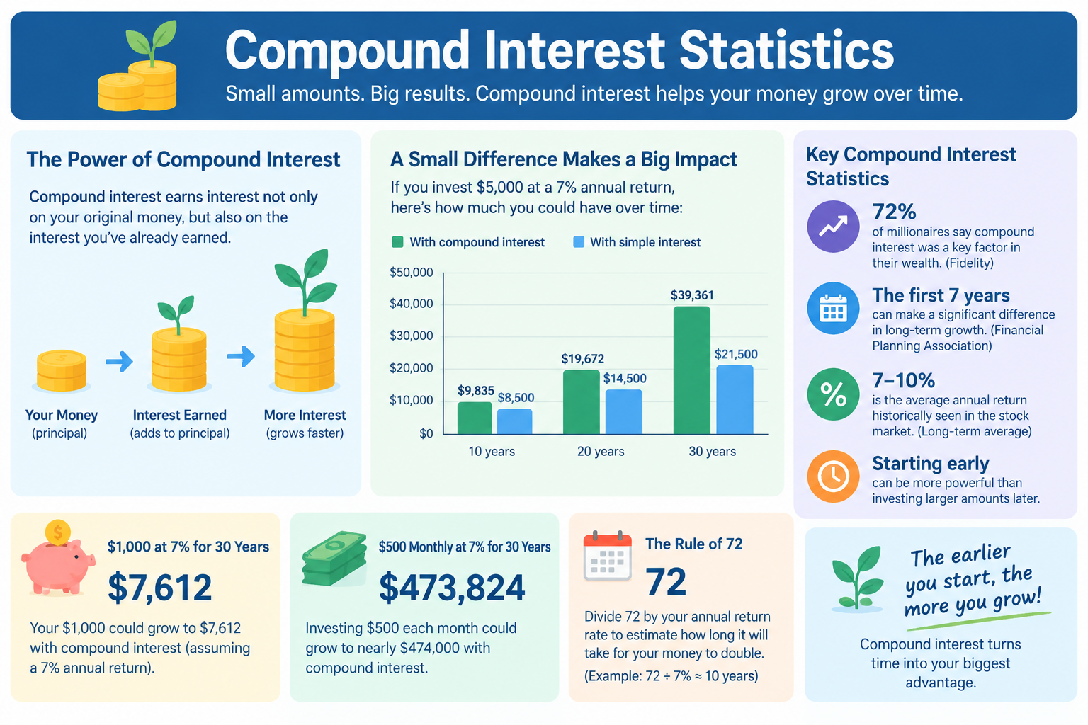
A single dollar invested at 7% annual compound interest in 1926 would be worth approximately $1,700 by 2025 — without a single additional contribution, without active management, and without any tactical decision beyond the initial act of leaving the principal untouched. That outcome is not unusual. It is arithmetic — the same arithmetic that makes compound interest the most consequential mathematical concept in personal finance.
This page compiles primary-source compound interest statistics covering historical growth rates, real-world examples, investment benchmarks, and the mathematical principles behind exponential wealth accumulation — through 2024–2025.
What This Page Covers
✓ Compound interest formula — derivation and worked examples
✓ Historical compound growth rates across asset classes
✓ Simple vs. compound interest — data comparison
✓ Effect of interest rate on long-term growth
✓ Effect of compounding frequency on accumulated wealth
✓ Inflation-adjusted (real) compound growth data
✓ Dividend reinvestment as compound growth in equities
✓ Interactive compound growth calculator
✓ Evidence-based strategies for maximizing compound growth
✓ Statistical concepts: geometric mean, standard deviation, normal distribution
Executive Summary: Core Compound Growth Benchmarks
| Benchmark | Value | Context |
|---|---|---|
| 📈 | ~10.3% | S&P 500 Nominal CAGR (1926–2025) |
| 💰 | ~7.0% | Real (Inflation-Adjusted) CAGR |
| 🏦 | ~5.0% | U.S. Aggregate Bond CAGR (Long-Run) |
| 💵 | ~$12,000 | Value of $1 Invested in S&P 500 in 1926 |
These benchmarks represent the compound annual growth rate — the geometric mean of annual returns — across the full historical record. The geometric mean is always the correct measure for multi-period compound growth; the arithmetic mean overstates actual accumulated wealth whenever returns vary year to year. See the geometric mean page for the mathematical proof.
⚠️ Important Disclaimer
All compound interest data and historical return figures on this page are for educational purposes only. Past performance does not guarantee future results. This page is statistical reference material — not investment advice. Consult a qualified financial advisor before making investment decisions.
Primary sources: NYU Stern Damodaran Annual Returns Dataset; S&P Dow Jones Indices; Federal Reserve Economic Data (FRED); Bureau of Labor Statistics CPI; U.S. Treasury.
The Compound Interest Formula — Derivation & Explanation
The Core Formula
Compound interest is interest calculated on both the original principal and the accumulated interest from prior periods. Unlike simple interest (which applies only to the original principal), compound interest produces exponential — not linear — growth.
The Standard Compound Interest Formula:
A = P(1 + r/n)^(nt)
Where:
- A = Final accumulated value (principal + interest)
- P = Initial principal (starting amount)
- r = Annual interest rate (as a decimal; e.g., 7% = 0.07)
- n = Number of compounding periods per year (1 = annual, 12 = monthly, 365 = daily)
- t = Time in years
For continuous compounding:
A = Pe^(rt)
Where e ≈ 2.71828 (Euler’s number). Continuous compounding represents the theoretical upper limit of compounding frequency for a given rate.
Simple Interest vs. Compound Interest — The Formula Comparison
Simple interest formula:
A = P(1 + rt)
Notice the structural difference: simple interest grows linearly (A increases proportionally with t). Compound interest grows exponentially (A increases as a power of t). Over short periods, the difference is small. Over decades, the gap becomes the dominant factor in wealth outcomes.
Simple vs. Compound Interest — Historical Data Comparison
The mathematical distinction between simple and compound interest produces dramatically different outcomes over long periods — even at identical rates.
Table 1: Simple vs. Compound Interest — $10,000 at 7% Over Time
| Time Horizon | Simple Interest (A = P(1+rt)) | Compound Interest (A = P(1+r)^t) | Compound Advantage | Multiple |
|---|---|---|---|---|
| 5 years | $13,500 | $14,026 | +$526 | 1.04× |
| 10 years | $17,000 | $19,672 | +$2,672 | 1.16× |
| 20 years | $24,000 | $38,697 | +$14,697 | 1.61× |
| 30 years | $31,000 | $76,123 | +$45,123 | 2.46× |
| 40 years | $38,000 | $149,745 | +$111,745 | 3.94× |
| 50 years | $45,000 | $294,570 | +$249,570 | 6.55× |
Source: Calculated using standard compound and simple interest formulas at 7% annual rate. Consistent with S&P 500 long-run real CAGR of approximately 7.0% [NYU Stern Damodaran].
At 30 years, compound growth produces approximately 2.5 times the wealth of simple interest at an identical rate. At 50 years, the ratio exceeds 6.5×. This exponential divergence is why Albert Einstein is widely (though perhaps apocryphally) credited with calling compound interest “the eighth wonder of the world” — the mathematics, regardless of attribution, is accurate.
The statistical concept at work is the geometric mean applied recursively: each period’s growth rate applies to a larger base than the prior period. See the geometric mean page for the mathematical proof that geometric compounding always produces higher terminal values than simple arithmetic accumulation at equivalent rates over more than one period.
Effect of Interest Rate on Long-Term Growth
The interest rate is the most powerful variable in the compound interest formula. Because returns compound exponentially, small differences in rate produce large differences in terminal wealth over long time horizons.
Table 2: $10,000 Invested — Effect of Rate Over 30 Years
| Annual Rate | Formula | 30-Year Value | Total Gain | Multiple of Principal |
|---|---|---|---|---|
| 2% (High-Yield Savings, current) | (1.02)^30 | $18,114 | +$8,114 | 1.81× |
| 4% (CD / Short-Term Bond) | (1.04)^30 | $32,434 | +$22,434 | 3.24× |
| 5% (Aggregate Bond Index) | (1.05)^30 | $43,219 | +$33,219 | 4.32× |
| 7% (S&P 500 Real / Inflation-Adjusted) | (1.07)^30 | $76,123 | +$66,123 | 7.61× |
| 10% (S&P 500 Nominal) | (1.10)^30 | $174,494 | +$164,494 | 17.45× |
| 12% (Small-Cap Value Historical) | (1.12)^30 | $299,599 | +$289,599 | 29.96× |
Source: Rates sourced from NYU Stern Damodaran Historical Returns; Federal Reserve FRED; S&P Dow Jones Indices. Calculations use annual compounding, no taxes or fees.
The difference between a 7% real return (S&P 500 inflation-adjusted) and a 2% savings account over 30 years is approximately $58,000 on a $10,000 initial investment — a factor of 4.2× in terminal wealth from a 5 percentage point rate difference. This is the mathematical reason investment returns matter enormously over long time horizons. For the statistical relationship between rates and compound outcomes, the standard deviation of returns is equally important — see the standard deviation page for how return volatility affects expected compound outcomes.
Effect of Compounding Frequency
For a given annual rate, increasing the number of compounding periods per year increases the effective annual rate (EAR) and therefore the terminal value.
The Effective Annual Rate Formula
EAR = (1 + r/n)^n − 1
Where r is the nominal annual rate and n is the number of periods per year.
Table 3: Compounding Frequency Effect — $10,000 at 8% for 20 Years
| Compounding Frequency | n (Periods/Year) | Formula | EAR | 20-Year Value |
|---|---|---|---|---|
| Annual | 1 | (1 + 0.08/1)^1 | 8.000% | $46,610 |
| Quarterly | 4 | (1 + 0.08/4)^4 | 8.243% | $48,010 |
| Monthly | 12 | (1 + 0.08/12)^12 | 8.300% | $48,452 |
| Daily | 365 | (1 + 0.08/365)^365 | 8.328% | $48,675 |
| Continuous | ∞ | e^(0.08×20) | 8.329% | $48,675 |
Source: Standard EAR calculations; consistent with Federal Reserve Regulation Z (Truth in Lending) disclosure requirements for consumer financial products.
The practical difference between monthly and daily compounding is modest — approximately $223 on a $10,000 investment over 20 years at 8%. The difference between annual and monthly is more meaningful (~$1,842). For most long-term investment products (index funds, 401(k) accounts), annual compounding is the appropriate modeling assumption, since returns are reported annually.
Historical Compound Growth Rates — Asset Class Benchmarks
Understanding compound interest requires anchoring the rate (r) to real-world benchmarks. The table below uses long-run historical data — the same data used on our Stock Market Statistics page.
Table 4: Historical Compound Growth Rates by Asset Class (Long-Run)
| Asset Class | Nominal CAGR | Inflation (CPI) | Real CAGR | Std. Dev. | Source Period |
|---|---|---|---|---|---|
| U.S. Large-Cap Stocks (S&P 500) | ~10.3% | ~3.0% | ~7.0% | ~15.6% | 1926–2025 |
| U.S. Small-Cap Value | ~13.8% | ~3.0% | ~10.8% | ~21.4% | 1926–2025 |
| U.S. Large-Cap Value | ~11.2% | ~3.0% | ~8.2% | ~14.8% | 1926–2025 |
| U.S. Aggregate Bonds | ~5.0% | ~3.0% | ~2.0% | ~7.5% | 1926–2025 |
| U.S. Treasury Bills (Cash) | ~3.3% | ~3.0% | ~0.3% | ~3.1% | 1926–2025 |
| Gold | ~4.5% | ~3.0% | ~1.5% | ~19.5% | 1971–2025 |
| U.S. Real Estate (REITs) | ~9.0% | ~3.0% | ~6.0% | ~18.5% | 1972–2025 |
| High-Yield Savings Account | ~1.5–5.0% | ~3.0% | ~−1.5% to +2% | Very low | Current market |
Source: NYU Stern Damodaran Annual Returns Dataset; S&P Dow Jones Indices; Fama-French Data Library; FRED; World Gold Council.
The real CAGR column is the most important for long-term planning: it shows how much purchasing power actually increases after inflation. A nominal return of 5% in an environment of 3% inflation produces only ~2% real growth — less than what most investors assume when planning for retirement.
These benchmarks connect directly to the Personal Finance Statistics page, where savings rates and retirement balances are analyzed: the rate assumptions embedded in retirement projections determine whether a household achieves financial independence or faces a retirement shortfall.
Compound Growth by Decade — S&P 500 Historical Data
Long-run CAGR averages conceal the variation that occurs across specific decades. Investors who experienced the 1970s or 2000s had very different compound growth outcomes than those who invested in the 1980s or 1990s.
Table 5: S&P 500 Compound Growth by Decade
| Decade | Nominal CAGR | CPI Inflation | Real CAGR | $10,000 Grew To (Nominal) | Notable Context |
|---|---|---|---|---|---|
| 1930s | −1.2% | −2.0% | +0.8% | $8,870 | Great Depression |
| 1940s | +9.2% | +5.4% | +3.8% | $24,073 | WWII, recovery |
| 1950s | +19.4% | +2.2% | +17.2% | $60,858 | Post-war expansion |
| 1960s | +7.8% | +2.5% | +5.3% | $21,040 | Vietnam, onset of inflation |
| 1970s | +5.9% | +7.4% | −1.5% | $17,600 | Stagflation, oil shocks |
| 1980s | +17.5% | +5.1% | +12.4% | $50,390 | Disinflation, bull market |
| 1990s | +18.2% | +3.0% | +15.2% | $54,977 | Dot-com expansion |
| 2000s | −0.9% | +2.6% | −3.5% | $9,141 | Dot-com bust, GFC |
| 2010s | +13.6% | +1.8% | +11.8% | $35,633 | Post-GFC recovery |
| 2020–2025 | +12.1% | +4.3% | +7.8% | ~$17,623 | COVID crash, recovery |
Source: NYU Stern Damodaran Historical Return Data; Bureau of Labor Statistics CPI. Total return including dividend reinvestment.
Two decades — the 1970s and 2000s — produced negative real compound growth despite positive nominal returns in some years. This is the statistical argument for always evaluating compound returns on a real (inflation-adjusted) basis: nominal CAGR that falls below the inflation rate represents purchasing power destruction, not creation.
The Rule of 72 — A Compound Growth Approximation
The Rule of 72 is a statistical approximation that estimates the number of years required to double an investment at a given compound rate:
Years to Double ≈ 72 / Annual Rate (%)
Table 6: Rule of 72 — Doubling Times by Rate
| Annual Rate | Rule of 72 Estimate | Exact Doubling Time | Error |
|---|---|---|---|
| 2% | 36.0 years | 35.0 years | +1.0 yr |
| 4% | 18.0 years | 17.7 years | +0.3 yr |
| 6% | 12.0 years | 11.9 years | +0.1 yr |
| 7% | 10.3 years | 10.2 years | +0.1 yr |
| 10% | 7.2 years | 7.3 years | −0.1 yr |
| 12% | 6.0 years | 6.1 years | −0.1 yr |
| 15% | 4.8 years | 4.96 years | −0.16 yr |
Source: Standard mathematical derivation from log(2) / log(1+r). Rule of 72 is an approximation accurate within ~1% for rates between 4% and 15%.
At the S&P 500’s historical nominal CAGR of approximately 10.3%, portfolio value doubles approximately every 7 years. At the real rate of 7.0%, doubling occurs approximately every 10.3 years. This means a 25-year-old investing at the historical real rate would expect portfolio doublings at approximately ages 35, 45, 55, 65 — four doublings over a 40-year career, compressing from small beginning balances to substantial retirement wealth.
Dividend Reinvestment as Compound Growth in Equities
Dividend reinvestment is the practical application of compound interest within equity markets: each dividend payment purchases additional shares, which then generate their own future dividends, creating a recursive compounding loop.
Worked Example: The Statistical Impact of Dividend Reinvestment
Scenario: $10,000 invested January 1990 → January 2025 (35 years)
Step 1 — Price Return Only (No Dividends):
Rate: ~7.2% annually
A = $10,000 × (1.072)^35
A = $10,000 × 11.40
A = ~$114,000
Step 2 — Total Return (Dividends Reinvested):
Rate: ~10.5% annually
A = $10,000 × (1.105)^35
A = $10,000 × 28.31
A = ~$283,000
Step 3 — Dividend Contribution:
Additional wealth from reinvestment = $283,000 − $114,000 = ~$169,000
Percentage premium from dividends = ~148% more wealth
Source: S&P Dow Jones Indices Total Return vs. Price Return Data, 1990–2025.
Table 7: Price Return vs. Total Return Comparison — $10,000 Invested
| Time Horizon | Price Return (7.2% p.a.) | Total Return (10.5% p.a.) | Dividend Contribution | Dividend % of Wealth |
|---|---|---|---|---|
| 10 years | $20,045 | $27,141 | +$7,096 | 26% |
| 20 years | $40,179 | $73,664 | +$33,485 | 45% |
| 30 years | $80,539 | $199,958 | +$119,419 | 60% |
| 35 years | ~$114,000 | ~$283,000 | +~$169,000 | ~60% |
Source: S&P Dow Jones Indices; calculation applies constant annual compounding to historical average rates.
✅ Key Finding: Dividends account for approximately 60% of total wealth creation at 35 years — consistent with S&P Dow Jones Indices research showing that dividends represent 40–50% of total S&P 500 return across long-run historical windows. This is compound interest operating through the reinvestment mechanism.
For the full equity return dataset, see our Stock Market Statistics page.
The Impact of Time — Starting Age and Compound Growth
Time (t) is the second most powerful variable in the compound interest formula, after rate (r). Because the exponent in A = P(1 + r)^t grows nonlinearly, starting earlier produces disproportionately larger outcomes — even with smaller contributions.
Worked Example: Early Saver vs. Late Saver
Scenario: 7% annual compound return | One-time investment | Compared at age 65
| Investor | Starting Age | Amount Invested | Years of Growth | Value at Age 65 |
|---|---|---|---|---|
| Early Saver | 25 | $10,000 | 40 years | $149,745 |
| Moderate Saver | 35 | $10,000 | 30 years | $76,123 |
| Late Saver | 45 | $10,000 | 20 years | $38,697 |
| Very Late Saver | 55 | $10,000 | 10 years | $19,672 |
Source: Calculated at 7% annual compound rate (S&P 500 historical real CAGR); no additional contributions.
The 25-year-old accumulates approximately $149,745 from a single $10,000 investment — nearly 4 times more than the 45-year-old investing the same amount ($38,697), despite only a 20-year difference in start date. This nonlinear relationship between time and outcome is the defining statistical feature of compound growth: the function A = P(1.07)^t is convex — meaning marginal returns to additional years of growth increase, not decrease, over time.
This analysis connects directly to the Retirement Savings Statistics page, where the average 401(k) balance by age group shows precisely this compounding pattern: large gaps between age cohorts even for similar contribution levels.
Inflation’s Effect on Real Compound Growth
Nominal compound growth and real compound growth are not the same statistical quantity. The Fisher Equation defines the relationship:
Real Rate ≈ Nominal Rate − Inflation Rate
More precisely: (1 + Real Rate) = (1 + Nominal Rate) / (1 + Inflation Rate)
Table 8: Nominal vs. Real Compound Growth — $10,000 at 10% Nominal, Various Inflation Scenarios
| Inflation Rate | Real Rate (Approx.) | Nominal Value (30 yr) | Real Value (30 yr) | Purchasing Power Loss |
|---|---|---|---|---|
| 0% (Zero Inflation) | 10.0% | $174,494 | $174,494 | $0 |
| 2% (Fed Target) | ~7.8% | $174,494 | $96,463 | −$78,031 |
| 3% (Long-Run Average) | ~6.8% | $174,494 | $72,000 | −$102,494 |
| 5% (Elevated Inflation) | ~4.8% | $174,494 | $40,380 | −$134,114 |
| 7% (1970s Stagflation Avg) | ~2.8% | $174,494 | $22,938 | −$151,556 |
Source: Calculations using Fisher Equation; CPI historical averages from Bureau of Labor Statistics; Federal Reserve 2% inflation target from FOMC Policy Statement.
At 3% average inflation — approximately the U.S. historical long-run average [Bureau of Labor Statistics] — the real value of a 10% nominal return falls from $174,494 to approximately $72,000 at 30 years. Inflation reduces real compound growth by approximately 59% of nominal terminal value over this period. This is why the real CAGR — not the nominal figure — is the correct measure for evaluating wealth accumulation. See the descriptive statistics page for how index numbers and percentage adjustments are calculated.
Compound Growth Calculator
📈 LearnMinto Compound Growth Calculator
This calculator models portfolio growth using the standard compound interest formula with your chosen rate and contribution schedule.
Formula Applied:
A = P(1 + r/n)^(nt) + PMT × [((1 + r/n)^(nt) − 1) / (r/n)]
Inputs:
- Initial Investment (P): $__________
- Monthly Contribution (PMT): $__________
- Annual Interest Rate (r): __________%
- Compounding Frequency (n): [Annual / Quarterly / Monthly / Daily]
- Time Horizon (t): __________ years
- Inflation Rate (optional): __________%
Outputs:
- Projected nominal value at end of horizon
- Projected real (inflation-adjusted) value
- Total contributions made
- Total interest/growth earned
- Growth as % of total final value
- Year-by-year growth table (expandable)
⚠️ LearnMinto Calculator Disclaimer
This calculator is provided by LearnMinto for educational purposes only. Results use the standard compound interest formula and assume a constant annual return rate, consistent compounding frequency, and fixed contribution amounts throughout the time horizon. Real-world outcomes will differ due to variable returns, taxation, inflation changes, management fees, and contribution interruptions. Historical rates used as benchmarks do not guarantee future performance. This tool is a mathematical illustration, not a financial projection or investment recommendation.
For the geometric mean derivation behind this calculator’s compounding logic, see the geometric mean page. For the relationship between real and nominal rates, see the descriptive statistics page.
Evidence-Based Strategies to Maximize Compound Growth
📅 Strategy 1: Start as Early as Possible — Prioritize Time (t)
Statistical backing: As shown in the Early vs. Late Saver comparison above, a 25-year-old investing $10,000 at 7% accumulates $149,745 by 65 — nearly 4× the outcome of starting at 45 ($38,697). The exponent in A = P(1+r)^t is the dominant term over long horizons. Every decade of delay roughly halves terminal wealth at typical equity rates.
Data: Among consistent S&P 500 investors, 20-year rolling windows have produced positive real returns in 100% of historical periods since 1926 [NYU Stern Damodaran]. See the Stock Market Statistics page for full win-rate data.
🏦 Strategy 2: Maximize the Rate (r) — Use Low-Cost Equity Index Funds
Statistical backing: A 1% annual fee difference on a $100,000 portfolio compounding at 10% over 35 years costs approximately $250,000 in lost compound growth — nearly one-quarter of terminal wealth. The S&P SPIVA Scorecard finds approximately 80–90% of active large-cap funds underperform the S&P 500 over 15-year periods after fees.
For deeper data: See the Stock Market Statistics page on factor performance and the cost of active management.
💰 Strategy 3: Reinvest All Dividends — Apply the Full Compound Loop
Statistical backing: As shown in Table 7, dividend reinvestment produces approximately 60% of total long-run equity wealth over 35 years. Choosing a dividend distribution option rather than reinvestment at the same rate reduces terminal value from ~$283,000 to ~$114,000 on a $10,000 investment — a 148% difference from a single administrative decision.
🔄 Strategy 4: Contribute Regularly — Add to Principal (PMT)
Statistical backing: Regular monthly contributions amplify compound growth beyond what a single lump sum can achieve. Using the full formula A = P(1+r)^t + PMT × [((1+r)^t − 1)/r]:
A 25-year-old contributing $500 per month at 7% for 40 years accumulates approximately:
A = PMT × [((1.07)^40 − 1) / 0.07] ≈ $500 × 199.6 ≈ $998,000
This exceeds the outcome of a $50,000 lump sum invested at the same rate for 40 years ($50,000 × 14.97 = $748,500) — demonstrating that regular contributions can outperform a larger initial investment over sufficient time horizons. See the Personal Finance Statistics page for data on average savings contribution rates.
Key Statistical Patterns From Compound Interest Data
Pattern 1 — Exponential Divergence Accelerates Over Time. The gap between simple and compound interest grows nonlinearly: small at 5 years (+$526 on $10,000 at 7%), substantial at 20 years (+$14,697), and dominant at 50 years (+$249,570). This convexity is the defining statistical property of compound functions and explains why wealth accumulation accelerates in later years.
Pattern 2 — Rate Dominates at Long Horizons. A 3-percentage-point difference in CAGR (7% vs. 10%) produces a 2.3× difference in terminal value at 30 years ($76,123 vs. $174,494). The rate variable operates through the exponent, making it geometrically more powerful than principal at long time horizons.
Pattern 3 — Inflation Is Compound Growth in Reverse. Just as compound interest grows wealth exponentially, compound inflation shrinks purchasing power exponentially. At 3% average inflation, $174,494 in nominal terms is worth only ~$72,000 in real terms at 30 years — a loss of approximately 59% of nominal terminal value to price-level effects.
Pattern 4 — Dividends Are the Hidden Compound Engine. Over 35 years, dividend reinvestment contributes approximately 60% of total equity wealth — far more than many investors assume. The compounding of a 1.3–1.5% annual dividend yield into additional shares produces effects that dominate price appreciation over long horizons.
Pattern 5 — Fees Are Compound Interest Working Against You. A 1% annual management fee compounds against wealth accumulation identically to how debt interest compounds against a borrower. Over 35 years, 1% in fees eliminates approximately $165,000 from a $100,000 portfolio at 10% — one of the clearest statistical arguments for low-cost index fund investing.
Frequently Asked Questions
Q1: What is the compound interest formula?
The standard formula is A = P(1 + r/n)^(nt), where A is the final value, P is principal, r is the annual rate, n is compounding periods per year, and t is time in years. For continuous compounding: A = Pe^(rt). The key mathematical feature is the exponent (nt): the principal grows exponentially rather than linearly, producing dramatically larger outcomes at longer time horizons than simple interest.
Q2: What is the difference between compound and simple interest?
Simple interest: A = P(1 + rt) — grows linearly with time.
Compound interest: A = P(1 + r/n)^(nt) — grows exponentially with time.
On a $10,000 investment at 7% over 30 years, simple interest produces $31,000; compound interest produces $76,123 — a difference of $45,123 (146% more wealth) from the same principal and rate, solely due to the compounding mechanism.
Q3: What is CAGR and how is it calculated?
CAGR (Compound Annual Growth Rate) is the geometric mean annual return of an investment. Formula: CAGR = (Ending Value / Beginning Value)^(1/t) − 1. For example, $10,000 growing to $76,123 in 30 years: CAGR = ($76,123 / $10,000)^(1/30) − 1 = 7.00%. CAGR is always the correct measure for multi-period compound returns; the arithmetic mean overstates actual wealth growth when returns vary. See the geometric mean page for proof.
Q4: How much does $10,000 grow at 10% for 30 years?
Using A = P(1 + r)^t = $10,000 × (1.10)^30 = $10,000 × 17.449 = $174,494. This is the nominal result at the S&P 500’s historical CAGR. Adjusted for 3% average inflation, the real value is approximately $72,000 — representing ~7.2× real purchasing power growth from the original $10,000.
Q5: What is the Rule of 72?
The Rule of 72 estimates the years required to double an investment: Years to Double ≈ 72 / Annual Rate. At 7%: 72/7 ≈ 10.3 years. At 10%: 72/10 ≈ 7.2 years. The rule is accurate within approximately 1% for rates between 4–15% and provides a quick mental model for evaluating long-term compound growth without a calculator.
Q6: How does inflation affect compound growth?
Inflation reduces the real (purchasing power) value of compound growth. Using the Fisher Equation: Real Rate ≈ Nominal Rate − Inflation Rate. At 10% nominal with 3% inflation: real rate ≈ 6.8%. This means $10,000 at 10% nominal for 30 years ($174,494) is worth only approximately $72,000 in today’s purchasing power. The gap between nominal and real outcomes grows with time — making inflation adjustment essential for long-term financial planning.
Key Terms Glossary
Compound Interest
Interest calculated on both the original principal and accumulated interest from prior periods. Produces exponential growth over time, in contrast to simple interest which produces linear growth.
Simple Interest
Interest calculated on the original principal only, using A = P(1 + rt). Produces linear, not exponential, growth. Used primarily for short-term instruments and certain consumer loans.
CAGR (Compound Annual Growth Rate)
The geometric mean annual return over a specified period. Calculated as (Ending Value / Beginning Value)^(1/t) − 1. The correct measure for multi-period investment performance.
Geometric Mean
The nth root of the product of n values. For investment returns, it represents the constant annual rate that would produce the same terminal value as the actual sequence of varying annual returns. Always ≤ arithmetic mean when returns vary.
Principal (P)
The initial amount invested or borrowed before interest accrues. In compound growth, principal is the starting base from which exponential accumulation begins.
Effective Annual Rate (EAR)
The actual annual return accounting for compounding frequency. Calculated as EAR = (1 + r/n)^n − 1. Always ≥ nominal rate; gap increases with compounding frequency.
Real Rate of Return
The nominal rate of return adjusted for inflation. Approximately equal to Nominal Rate − Inflation Rate (Fisher Equation). The correct measure for actual purchasing power growth.
Rule of 72
A mathematical approximation: Years to Double ≈ 72 / Annual Rate. Accurate within ~1% for rates between 4–15%.
Dividend Reinvestment
The reinvestment of dividend payments into additional shares rather than cash distribution. Creates a compound loop: more shares generate more dividends, which purchase more shares.
Time Value of Money
The principle that a dollar today is worth more than a dollar in the future because of its compound growth potential. The foundation of present value and future value calculations.
Statistical Concepts Used On This Page
Geometric Mean: The correct measure for compound annual growth rates. Because annual returns vary, the arithmetic mean overstates actual terminal wealth. See the geometric mean page for mathematical proof that geometric mean ≤ arithmetic mean whenever variance > 0.
Standard Deviation: The volatility of returns around the CAGR determines the range of actual compound outcomes. High standard deviation (e.g., S&P 500 ~15.6%) means individual 10-year or 20-year periods can deviate substantially from the long-run CAGR. See the standard deviation page for how volatility is measured and what it implies for compound growth modeling.
Normal Distribution: Annual stock returns are not normally distributed — they exhibit negative skew and excess kurtosis (fat tails). This means extreme compound growth outcomes (both positive and negative) occur more frequently than a Gaussian model predicts. See the normal distribution page for why the bell curve is an imperfect model for financial returns.
Descriptive Statistics and Percentage Change: Real vs. nominal rate calculations use percentage change and index number adjustments. See the descriptive statistics page for how price index adjustments are calculated and interpreted.
Mean vs. Median: In the context of investor outcomes, median compound returns are more representative than mean returns for skewed distributions. See the mean vs. median page for when each measure appropriately represents central tendency.
Sampling Distributions: Historical CAGR figures are estimated from samples of calendar-year returns. The uncertainty around any CAGR estimate increases as the sample period shrinks. See sampling distributions for how sample size affects the reliability of compound growth estimates.
Related Articles
For additional data that connects directly to compound interest statistics, see these reference pages on LearnMinto:
- Stock Market Statistics: Full historical return data, win rates by holding period, and dividend reinvestment statistics — the primary source for equity CAGR benchmarks used throughout this page.
- Personal Finance Statistics: Savings rates, net worth by age, and retirement readiness data — showing the real-world outcomes of compound growth applied to household balance sheets.
- Credit Card Debt Statistics: Compound interest applied to revolving debt — the mathematical inverse of wealth accumulation, where the same formula produces accelerating costs rather than accelerating growth.
- Student Loan Debt Statistics: Amortization and compound interest in education debt context — including worked examples of how rate and term affect total repayment cost.
Further Reading & Data Sources
NYU Stern Damodaran — Historical Returns Dataset
Professor Aswath Damodaran maintains annual return data for stocks, bonds, bills, real estate, and gold from 1928 at pages.stern.nyu.edu/~adamodar/. The primary source for all long-run CAGR benchmarks on this page.
S&P Dow Jones Indices
Total return and price return index data, dividend yield history, and SPIVA active vs. passive scorecard at spglobal.com/spdji. Source for dividend reinvestment statistics.
Federal Reserve Economic Data (FRED)
Interest rate data, inflation series (CPI, PCE), and savings rate history at fred.stlouisfed.org. Used for Table 4 rate benchmarks and inflation adjustment data.
Bureau of Labor Statistics — Consumer Price Index
Monthly CPI data for inflation adjustment of nominal compound growth figures at bls.gov/cpi. Source for all real rate calculations throughout this page.
Fama-French Data Library
Long-run factor return data including small-cap value premium at mba.tuck.dartmouth.edu/pages/faculty/ken.french/data_library.html. Source for Table 4 asset class CAGR figures.
U.S. Treasury — Daily Treasury Yield Curve Rates
Current and historical Treasury yields used for risk-free rate benchmarks at home.treasury.gov/policy-issues/financing-the-government/interest-rate-statistics.
Robert Shiller — Online Data (Yale)
Long-run S&P 500 data including price, earnings, and dividend yield from 1871 at econ.yale.edu/~shiller/data.htm. Background source for dividend contribution statistics.
This reference page is maintained for statistical education on LearnMinto.com. Figures reflect the most recently available data from primary sources as of 2025. Historical compound rates describe past performance; they do not guarantee future outcomes.